The Large-Scale Variability Model

In the MCD, data are stored in 12 seasonal bins and at 12 local times of day within each season. Although this captures the main seasonal and diurnal components of variability, any intra-seasonal or day-to-day (synoptic) variations are averaged out. Thus there is a need to simulate this variability, especially if the user wishes to produce an ensemble of realizations of a variable at a particular seasonal date and local time of day which covers a realistic range of variability.

In version 1.0 of the MCD large-scale variability in a vertical profile of a meteorological variable, D(z), was modelled by adding a series of functions to a mean vertical profile, $\overline{D}(z)$, 

$$D(z)~=\overline{D}(z)~+~\sum_{i=1}^N~p_i {\bf e}_i(z)$$ (6)

where the functions ${\bf e}_i(z)$ are eigenvectors of the covariance matrix of all the pre-averaged profiles generated by the GCM and p_i are the amplitudes of the functions. The eigenvectors, ${\bf e}_i$, are often called Empirical Orthogonal Functions (EOFs) and the p_i are referred to as the Principal Components (PCs) (see, e.g. North, 1984; Mo and Ghil, 1987). The set $\{{\bf e}_i\}$ form an optimal linear basis such that the variance capture is high even when the truncation limit is low.

Horizontal Correlations

In version 1.0 only correlations in altitude between variables were considered when calculating the covariance matrix. However, in order to retain cross-correlations between different variables (zonal wind, meridional wind, temperature, surface pressure and density) all were normalized and combined together to form a set of multivariate functions. Different sets of EOFs were computed for each of the 12 seasons on a low resolution grid (20$^\circ$ longitude $\times$ 20$^\circ$latitude) and the series (6) was truncated at N=6 to reduce the demands on data storage. Even so, typically $80-90\%$ of the variance was retained in the version 1.0 variability model at this level of truncation.

In order to improve the model it is desirable to extend the spatial dimension to include correlations between variables in both the horizontal and the vertical. Ultimately it would be desirable to include all the longitude, latitude and vertical grid-points in the analysis. A technical point, however, must be noted here. In computing the EOFs, the eigenvalues and eigenvectors of an $N \times N$ real symmetric matrix must be found. The order, N, of the matrix depends on the number of variables and on the number of spatial points. Since the number of calculations needed to perform the eigenvector problem increases as N³ there is a limit on the value of N that can be handled practically. The estimated CPU time and storage requirements for calculating the eigenvectors of the full problem (even on the low resolution grid with four three-dimensional and one two-dimensional variables, for which $N=18 \times 9 \times (4 \times 25+1)=16362$) is prohibitive.

We make the choice, therefore, to calculate EOFs in the two-dimensional, height-longitude plane which gives a manageable set of eigenvector problems. There is some physical basis for this choice, in that much of the variability the model must account for is in the form of baroclinic waves which, in general, propagate West to East along lines of latitude.

Statistical Stability and PC Modelling

In version 1.0 of the MCD we calculated separate sets of the variability EOFs for each of the 12 seasons. However, due to the relatively small number of days in each season (50-70), this can lead to poor estimation of the EOFs. Greater statistical stability can be achieved by forming the covariance matrix over the entire annual cycle, although this means that more EOFs must be retained in the series (6) in order to still capture a relatively high fraction of the variance. Fortunately this is possible as there is then no need to store the EOFs at each season. In fact the series can be extended to include 72 ($=12 \times 6$) EOFs rather than just 6 per season with no increase in the amount of space needed to store the MCD.

This also overcomes a problem which might occur with the version 1.0 implementation of the PC modelling. If a time series of a variable was computed across a seasonal boundary there could be a discontinuity at the boundary where the quadratic fit to the intra-seasonal or trend components did not match. In the improved version 2.0 of the variability model we simply store a smooth version of each PC to represent the seasonal cycle together with a variance to represent synoptic activity. This both simplifies and improves the algorithm.

Calculation of EOFs and PCs

Consider a time series of longitude-pressure vectors of zonal wind, ${\bf u}(\phi,p,t)$, meridional wind, ${\bf v}(\phi,p,t)$, temperature, ${\bf T}(\phi,p,t)$, density, ${\bf \rho}(\phi,p,t)$ and surface pressure $p^*(\phi,t)$ at M discrete time points and on L spatial points. We form a time series of vectors ${\bf D}(t)$, where

$${\bf D}(t)~=~(\hat{\bf u}(\phi,p,t), \hat{\bf v}(\phi,p,t), ... ...\bf T}(\phi,p,t), \hat{p^*}(\phi,t), \hat{\bf \rho}(\phi,p,t))$$ (7)

and the hat $\hat{}$ denotes a removal of the series mean and normalization of variance operator,

$$\overline{u}~=~\frac{1}{ML}\sum_{m=1}^M \sum_{l=1}^L u_{ml}$$ (8)

$$\hat{u}_{ml}~=~\frac{u_{ml}-\overline{u}} {\sqrt {\frac{1}{ML}\sum_{m=1}^M \sum_{l=1}^L (u_{ml}-\overline{u})^2}}$$ (9)

where the m denotes time and the l denotes spatial point. Hence, with this normalization, the variance of the entire time series of ${\bf D}(t)$ is unity.

We then form the $(N \times N)$ covariance matrix, ${\bf C}$, such that

$${\bf C}~=~\frac{1}{N}{\bf D}{\bf D}^T$$ (10)

where N= (number of horizontal points) $\times$ (4 $\times$ number of vertical points + 1), ${\bf D}$ is the $(N \times M)$ matrix whose rows are the vectors ${\bf D}(t)$ and the superscript T indicates the transpose.

The matrix ${\bf C}$ is real symmetric and we can find the eigenvectors and eigenvalues and order them in decreasing eigenvalue magnitude. We note that if ${\bf E}_i$ is the ith eigenvector then

$$\vert{\bf E}_i\vert~=~1$$ (11)

where $\vert\cdot\vert$ is the Euclidean Norm, and

$$\sum_{i=1}^N \lambda_i~=~1$$ (12)

where $\lambda_i$ is the ith eigenvalue.

The ith principal component (PC) at time m, p_mi is defined as

$$p_{mi}~=~\sum_{n=1}^N D_{mn} E_{ni}~=~{\bf D}\cdot{\bf E}_i$$ (13)

and we note the result

$$\frac{1}{MN}\sum_{m=1}^M (p_{mi})^2~=~\lambda_i$$ (14)

Each principal component has 669 values during one year (one per day). From the PCs we calculate a 30 day running mean, ps_mi, and a variance departure from that mean, pv_mi. The modelled PC, p'_mi, at time m is then  

$$p'_{mi}~=~ps_{mi}+\Phi pv_{mi}$$ (15)

where $\Phi$ is a normally distributed random variable with unit standard deviation.

Variance Capture

In version 1.0 of the variability model only 6 EOFs per location per season were retained in the series in Equation 6 to limit the amount of data storage required. Because, in the improved version, a single set of EOFs are calculated for the whole year, 72 EOFs can be retained in the series with no greater storage overhead, to give a potentially greater overall variance capture. Figure 5 shows the fraction of variance captured by retaining 72, 36, 18 and 9 EOFs at different latitudes. By retaining 36 EOFs approximately 90% or greater of the variance is captured and by retaining 72 EOFs approximately 95% or greater of the variance is captured. Including more EOFs gives relatively little increase in variance capture but increases the storage requirements considerably. Thus 72 EOFs seems to be a good compromise between variance capture and data storage.

 

Figure 5: The fraction of variance captured by 72 EOFs (squares), 36 EOFs (triangles), 18 EOFs (plus signs) and 9 EOFs (diamonds) at different latitudes for the Viking scenario run. 72 EOFs capture more than 95% of the variance at most latitudes. 

Examples of Cross-Sections

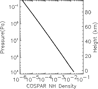
Density is one of the most important variables used by engineers in mission planning (e.g. when calculating entry trajectories or aerobraking manoeuvres). Hence the new variability model is illustrated using this field. Because density varies exponentially with height it is useful to compare any density profile with some `standard' profile. Figure 6 shows the northern hemisphere COSPAR standard atmospheric density profile from the surface to approximately 90 km. All density profiles are referenced to this profile by expressing the density as a percentage difference, d, from the COSPAR profile. i.e.

$$d~=~100\times\frac{~\rho_{COSPAR}-\rho}{\rho_{COSPAR}}$$ (16)

 

Figure 6: COSPAR northern hemisphere mean density (kgm^-3) for Mars. Note the logarithmic scale on the abscissa. 

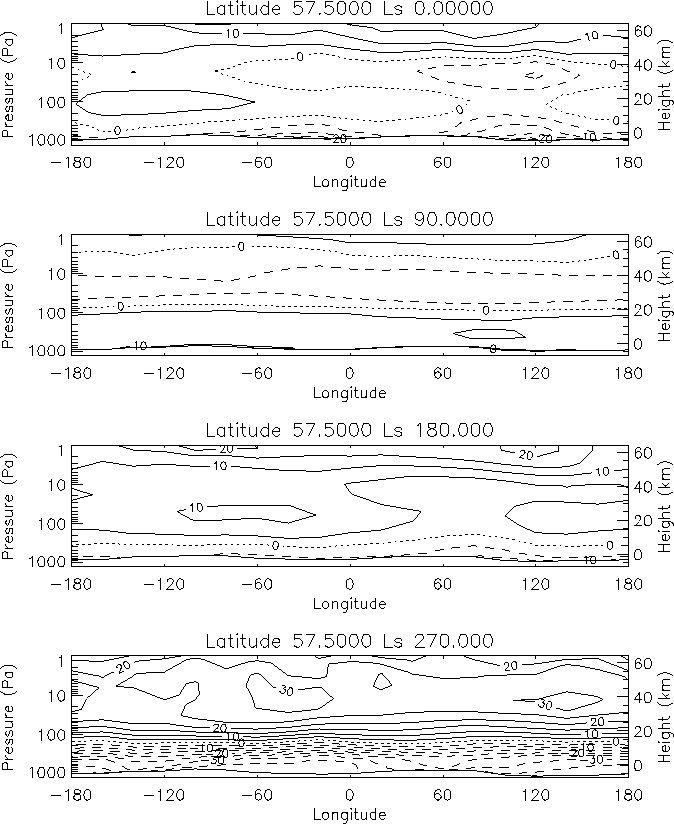
Figure 7 shows a selection of instantaneous longitude-height fields of density (referenced to the COSPAR profiles) taken directly from the Viking scenario GCM run at $L_S=0^\circ$,$L_S=90^\circ$, $L_S=180^\circ$ and $L_S=270^\circ$. The variability model simulations of these fields are shown in Figure 8. On a large scale the variability model captures the seasonal cycle of density variability well. Small differences between the GCM and the variability model simulated fields are due to the random nature of the PC model (Equation 15).

 

Figure 7: Longitude-height cross sections of density at 57.5$^\circ$N expressed as a deviation from the COSPAR northern hemisphere reference profile at several seasonal dates. The fields are instantaneous and have been taken from the Viking scenario GCM run. 

 

Figure 8: Longitude-height cross sections of density at 57.5$^\circ$N simulated using the new variability model and expressed as a deviation from the COSPAR northern hemisphere reference profile.