The Small-Scale Variability Model

The small-scale variability model simulates perturbations of density, temperature and wind due to the upward propagation of small-scale gravity waves. The model is based on the parameterization scheme used in the numerical models that simulated the data in the database (see Collins et. al, 1997).

The surface stress exerted by a vertically-propagating, stationary gravity wave can be written

$$\tau_0~=~\kappa \rho_0 N_0 \vert{\bf v_0}\vert \sigma_0$$ (17)

where $\kappa$ is a characteristic gravity wave horizontal wave number, $\rho_0$ is the surface density, N₀ is the surface Brunt Väisälä frequency, ${\bf v_0}$ is the surface vector wind and $\sigma_0$ is a measure of the orographic variance. In this case we choose the model sub-grid scale orographic variance. The surface stress can be related to the gravity wave vertical isentropic displacement, $\delta h$, by

$$\tau_0~=~\kappa \rho_0 N_0 \vert{\bf v_0}\vert \delta h^2.$$ (18)

We then assume that the stress, $\tau$, above the surface is equal to that at the surface. This leads to an expression for $\delta h$, at height z,

$$\delta h~=~\sqrt{\frac{\rho_0 N_0 \vert{\bf v_0}\vert \sigma_0} {\rho N \vert{\bf v}\vert}}$$ (19)

where $\rho$, N and ${\bf v}$ are the density, Brunt Väisälä frequency and vector wind at height z.

The gravity wave perturbation to a meteorological variable is calculated by considering vertical displacements of the form

$$\delta z = \delta h \sin \left(\frac{2 \pi z}{\lambda} + \phi_0 \right)$$ (20)

where $\lambda$ is a characteristic vertical wavelength for the gravity wave and $\phi_0$ is a randomly generated surface phase angle. Perturbations to temperature, density and wind at height z are then found by using the value at $z + \delta z$ on the background profile, with the perturbations to temperature and density calculated on the assumption of adiabatic motion to the valid height. 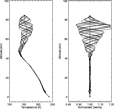A value can be chosen for $\lambda$to provide a reasonable comparison with the observed Viking entry temperature profiles above 50km; we take $\lambda=16$km. An example of several small scale perturbations is shown in Figure 9.

 

Figure 9: A series of ten perturbations generated by the small scale variability model added to mean profiles of temperature and density from the MCD; these correspond to the Viking Lander 1 entry location and time.